4. 密度プロット#
4.1. 概要#
密度プロット(Density Plot) とは,主に量的変数に対して,分布の形状をカーネル密度推定による 曲線 で表現するグラフです. ヒストグラムより滑らかに分布を表現することが可能ですが,あくまでも推定結果であることに注意が必要です.
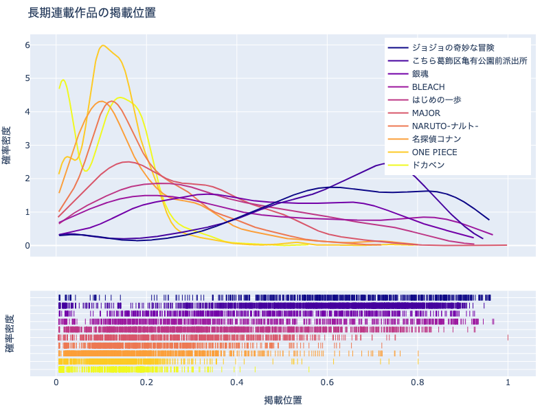
例えば上図は,作品ごとの掲載位置の分布(の推定値)を表現した密度プロットです.ヒストグラムと異なり,複数の分布を重ねて表示できることがわかります.
4.2. Plotlyによる作図方法#
Plotlyでは,plotly.figure_factory.create_distplot()で密度プロットを作成可能です.
import plotly.figure_factory as ff
fig = ff.create_distplot(
[hist_data, labels, show_hist=False)
ただし,hist_dataは描画したい変数ごとの変数のリスト,labelsは凡例名のリストを表します.hist_dataの要素数と,labelsの要素数は一致している必要があるのでご注意ください.
show_hist=False
plotly.figure_factory.create_distplot()はデフォルト設定でヒストグラムとDensity plotの両方を作図します.Density plotのみ表示したい場合は,show_hist=Falseを指定しましょう.
4.3. MADB Labを用いた作図例#
4.3.1. 下準備#
import pandas as pd
import plotly.figure_factory as ff
import plotly.express as px
import warnings
warnings.filterwarnings('ignore')
# 前処理の結果,以下に分析対象ファイルが格納されていることを想定
PATH_DATA = '../../data/preprocess/out/episodes.csv'
# Jupyter Book用のPlotlyのrenderer
RENDERER = 'plotly_mimetype+notebook'
# 平均掲載位置を算出する際の最小連載数
MIN_WEEKS = 5
def show_fig(fig):
"""Jupyter Bookでも表示可能なようRendererを指定"""
fig.update_layout(margin=dict(t=50, l=25, r=25, b=25))
fig.update_layout(legend={
'yanchor': 'top',
'xanchor': 'right',
'x': 0.99, 'y': 0.99})
fig.show(renderer=RENDERER)
df = pd.read_csv(PATH_DATA)
4.3.2. 長期連載作品の掲載位置の分布#
合計連載週数が多い10作品に対して,同様に分布を図示してみましょう.
df_tmp = \
df.groupby('cname')['pageStartPosition']\
.agg(['count', 'mean']).reset_index()
df_tmp = \
df_tmp.sort_values('count', ascending=False, ignore_index=True)\
.head(10)
cname2position = df_tmp.groupby('cname')['mean'].first().to_dict()
df_plot = df[df['cname'].isin(list(cname2position.keys()))]\
.reset_index(drop=True)
df_plot['position'] = df_plot['cname'].apply(
lambda x: cname2position[x])
df_plot = df_plot.sort_values('position', ignore_index=True)
cnames = df_tmp.sort_values('mean')['cname'].values
data = [
df[df['cname']==cname].reset_index(drop=True)\
['pageStartPosition'] for cname in cnames]
fig = ff.create_distplot(
data, cnames, show_hist=False,
colors= px.colors.sequential.Plasma_r)
fig.update_xaxes(title='掲載位置')
fig.update_yaxes(title='確率密度')
fig.update_layout(
hovermode='x unified', height=600,
title_text='長期連載作品の掲載位置')
show_fig(fig)
ヒストグラムと異なり,複数の凡例を同時に表示できるため,比較が楽です.
4.3.3. 長期連載作品の話数毎の掲載位置の分布#
# 話数の区切り
UNIT_EP = 200
cnames = df_tmp.sort_values('mean')['cname'].values
for cname in cnames:
df_c = df[df['cname']==cname].reset_index(drop=True)
df_c['eprange'] = (df_c.index + 1) // UNIT_EP * UNIT_EP
eps = sorted(df_c['eprange'].unique())
data = [
df_c[df_c['eprange']==e]['pageStartPosition']
for e in eps]
labels = [f'{e}話以降' for e in eps]
fig = ff.create_distplot(
data, labels, show_hist=False,
colors= px.colors.sequential.Plasma_r)
fig.update_xaxes(title='掲載位置')
fig.update_yaxes(title='確率密度')
fig.update_layout(
hovermode='x unified', height=500,
title_text=f'{cname}の掲載位置')
show_fig(fig)