Quantitative Evaluation of Tile Placement and Angle Assignment Strategies for Automatic Kakeami Generation
Abstract
Kakeami is a traditional manga shading technique in which small rectangular tiles are filled with parallel hatching lines at varying angles to create tonal gradation. We propose an automatic generation algorithm combining Poisson-disk tile placement, Voronoi adjacency construction, and BFS greedy angle assignment, which produces the most natural-looking kakeami among all tested conditions by visual inspection. To evaluate this claim quantitatively, we introduce eight complementary quality metrics — angle contrast ($E_{\mathrm{contrast}}$), angle entropy ($H_{\mathrm{angle}}$), angle autocorrelation at graph distances 1–3 ($R_1$, $R_2$, $R_3$), correlation length ($\xi$), coverage ratio ($C_{\mathrm{cov}}$), and Voronoi cell area CV ($U_{\mathrm{vor}}$) — and conduct a controlled 2×2 factorial experiment with 100 random seeds, supplemented by a deterministic grid-checkerboard reference condition.
The proposed condition does not rank first on any of the eight metrics. The checkerboard achieves the highest $E_{\mathrm{contrast}}$ despite looking mechanical; random-angle conditions achieve the highest $H_{\mathrm{angle}}$ while lacking consistent local contrast. Two-way ANOVA confirms that angle assignment is the dominant factor ($\eta^2 \approx 0.94$ for $E_{\mathrm{contrast}}$) and the metrics are useful for component-level ablation, but they fail to capture the holistic visual quality — the “grain” — that distinguishes natural-looking kakeami from mechanical or random patterns. Defining a metric that aligns with subjective kakeami quality remains an open problem.
1. Introduction
Kakeami (カケアミ) is a shading technique in Japanese manga. Small blocks are filled with parallel hatching lines, and adjacent blocks use different angles to create tonal gradation (Pixiv Encyclopedia; Toudo, 2003). The technique has a hierarchy of density: 1-kake (single direction), 2-kake (perpendicular overlay at 90°), 3-kake (adding a 45° diagonal), and 4-kake (four directions at 45° intervals).
Unlike Western cross-hatching, where long strokes traverse entire regions along contour or principal curvature directions, kakeami uses a fragmented patch structure: each tile is a small, self-contained unit whose orientation is chosen to contrast with its neighbours (Japanese with Anime).
Despite its importance in manga production, no academic paper has formally defined kakeami or evaluated automatic generation algorithms quantitatively. We identify five properties of good kakeami: (1) local angular contrast — neighbouring tiles should differ in angle; (2) angle diversity — a rich variety of orientations, not just two; (3) spatial coverage — no visible gaps between tiles; (4) spatial uniformity — evenly distributed tile centres; and (5) aperiodicity — no long-range periodic repetition of angles. This last property distinguishes natural-looking kakeami from mechanical patterns like a checkerboard. We propose a multi-metric framework that independently measures each property and a controlled 2×2 factorial experiment evaluating two independent components of a proposed algorithm: tile placement (Poisson-disk vs. uniform random) and angle assignment (BFS greedy vs. random).
A central finding of this work is that while the proposed Poisson-disk + BFS greedy algorithm produces subjectively superior kakeami — with angular contrast visible everywhere and a natural “grain” that avoids mechanical repetition — none of the eight proposed metrics ranks it first. This reveals a fundamental gap between formal quality measures and human visual judgement.
The remainder of the report is organised as follows. Section 2 reviews related work in NPR hatching and manga generation to identify the gap this work addresses. Section 3 introduces a novel mathematical formulation for kakeami quality, drawing on concepts from spatial statistics, direction field theory, and condensed matter physics. Section 4 describes the proposed algorithm and the baseline conditions. Section 5 details the experimental setup, Section 6 presents the quantitative results, Section 7 discusses their implications — including the gap between metrics and subjective quality — Section 8 outlines directions for future work, and Section 9 concludes.
2. Related Work
To situate our contribution, we survey three lines of prior work: classical NPR hatching, ML-based manga generation, and aperiodic tiling theory. In each case, we highlight what existing approaches optimise and where kakeami-specific generation remains unaddressed.
2.1 NPR Hatching
Praun et al. (2001) introduced Tonal Art Maps for real-time hatching in non-photorealistic rendering (NPR). Their approach aligns strokes along principal curvature directions, prioritising smoothness. Hertzmann & Zorin (2000) similarly optimise direction fields for illustrative hatching on 3D surfaces. Our approach inverts this paradigm: kakeami requires contrast maximisation between adjacent tiles, making neighbouring angles as different as possible.
2.2 ML-Based Manga Tone Generation
Recent work uses machine learning for manga screentone generation: ScreenVAE (Xie et al., SIGGRAPH Asia 2020), Zhang et al. (CVPR 2021), and Sketch2Manga (2024). These are data-driven and provide limited user control over geometric parameters. A purely geometric, controllable approach to kakeami-specific hatching remains unexplored.
2.3 Aperiodic Tilings in NPR
The Pinwheel tiling (Conway & Radin, 1998) provides aperiodic tessellations with infinite rotational diversity. While studied in mathematical tiling theory, no prior application to NPR hatching has been reported.
2.4 Direction Field Design
In geometry processing, direction fields on meshes are optimised using Ginzburg–Landau energy functionals (Beaufort et al., 2017; Viertel & Osting, 2019), primarily for quad meshing rather than artistic hatching. The connection between direction fields and nematic liquid crystals is well known in physics (both deal with headless directors on manifolds), but no prior work applies this framework to evaluate or generate kakeami patterns.
2.5 Our Contribution
The combination of Poisson-disk sampling for tile placement, Voronoi adjacency graph construction, and BFS greedy angle optimisation has no precedent in the literature. This report provides the first quantitative ablation study of these components using quality metrics newly proposed for kakeami evaluation.
3. Formulation
The related work reveals a clear gap: no formal framework exists for defining what makes a kakeami pattern “good.” In this section, we propose a novel mathematical formulation that addresses this gap. The data structures (Section 3.2) mirror the manual drawing process, while the quality metrics (Section 3.3) are original contributions of this work, capturing the five key properties of good kakeami identified in Section 1 — local angular contrast, angle diversity, aperiodicity, spatial coverage, and spatial uniformity.
3.1 Angle Space
A fundamental observation is that hatching lines at 0° and 180° are visually identical. This motivates modelling orientations on the real projective line: $\Omega_\theta = \mathbb{RP}^1 \cong [0, \pi)$, with the Fubini–Study distance $d_{\mathbb{RP}^1}(\theta_1, \theta_2) = \min(|\theta_1 - \theta_2| \bmod \pi,\; \pi - |\theta_1 - \theta_2| \bmod \pi)$. This identification, standard in the $N$-RoSy direction field literature (Vaxman et al., 2016), is what enables us to define meaningful distance-based quality metrics below.
3.2 Data Structure Hierarchy
We define a hierarchy that mirrors the manual kakeami drawing process:
- A Stroke $\sigma = (\theta, \delta)$ specifies an orientation $\theta \in \mathbb{RP}^1$ and a line pitch $\delta > 0$.
- A Block $\beta$ groups a primary stroke with optional secondary strokes (for $k$-kake layering).
- A Tile $\tau = (c, \beta)$ places a block at centre $c \in \mathbb{R}^2$.
- A KakeamiConfig $K = \{\tau_1, \ldots, \tau_n\}$ is a finite set of tiles covering a rectangular region.
3.3 Quality Metrics
Given a configuration $K$ and its adjacency edge set $E$ (Voronoi adjacency edges derived from Delaunay triangulation of tile centres), we propose eight metrics split across three axes: two angular metrics evaluating local orientation quality, two aperiodicity metrics detecting long-range periodic repetition, and two spatial metrics evaluating placement quality. Together they independently measure the five properties of good kakeami (Section 1). To the best of our knowledge, these metrics have not been previously defined for hatching evaluation.
Angular Metrics
Angle Contrast $E_{\mathrm{contrast}}$
The most direct measure of kakeami quality: the normalised mean RP¹ distance over all adjacency edges. $$E_{\mathrm{contrast}} = \frac{2}{\pi |E|} \sum_{(i,j) \in E} d_{\mathbb{RP}^1}(\phi_i, \phi_j) \;\in [0, 1]$$ where $\phi_i$ is the primary angle of tile $i$. Higher values indicate better angle separation between neighbours, which is the defining visual characteristic of kakeami.
Angle Entropy $H_{\mathrm{angle}}$
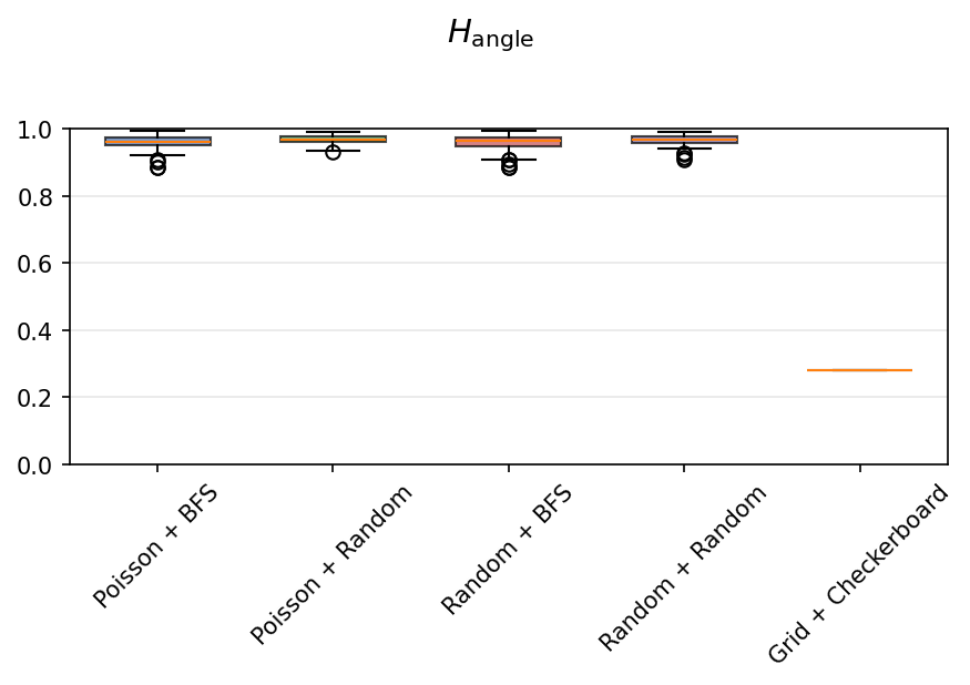
The normalised Shannon entropy of the primary-angle distribution measures how diverse the angle usage is across all tiles: $$H_{\mathrm{angle}} = -\frac{1}{\ln N_{\mathrm{bins}}} \sum_{b=1}^{N_{\mathrm{bins}}} p_b \ln p_b \;\in [0, 1]$$ where the angle range $[0, \pi)$ is divided into $N_{\mathrm{bins}} = 12$ equal bins (15° each) and $p_b$ is the fraction of tiles whose primary angle falls in bin $b$. $H_{\mathrm{angle}} = 1$ indicates a perfectly uniform distribution of angles across all bins; $H_{\mathrm{angle}} = 0$ means all tiles share the same angle. A checkerboard pattern using only 0° and 90° achieves $H_{\mathrm{angle}} = \ln 2 / \ln 12 \approx 0.28$, revealing its limited angle diversity.
Aperiodicity Metrics
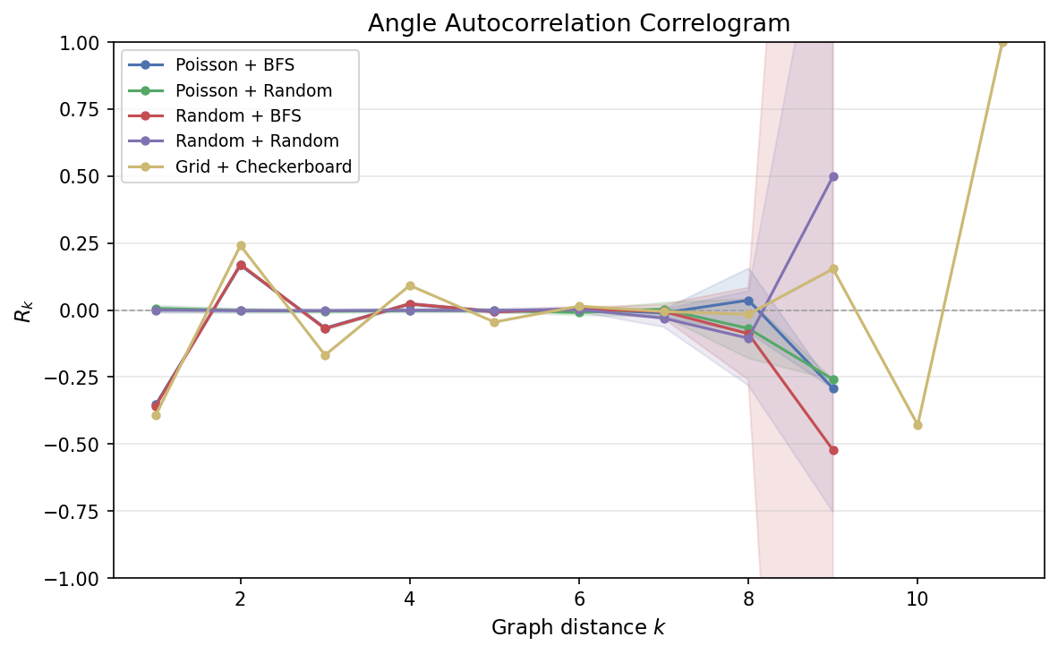
Angle Autocorrelation $R_k$
To detect long-range periodic repetition of angles, we define the angle autocorrelation at graph distance $k$: $$R_k = \frac{1}{|E_k|} \sum_{(i,j) \in E_k} \cos 2(\phi_i - \phi_j) \;\in [-1, 1]$$ where $E_k$ is the set of tile pairs at graph distance exactly $k$ (computed via BFS on the adjacency graph). $R_k = +1$ indicates that tiles at distance $k$ share the same angle (periodic repetition); $R_k = -1$ indicates perpendicular alignment; $R_k \approx 0$ indicates no angular correlation at distance $k$ (aperiodic). For kakeami, $|R_k| \approx 0$ for $k \geq 2$ is desirable — good local contrast ($R_1 \approx -1$) should not produce long-range patterns. We report the full correlogram $R_1, R_2, \ldots, R_D$ where $D$ is the graph diameter (capped at 15).
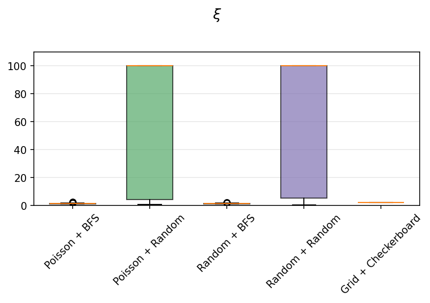
Correlation Length $\xi$
To quantify the spatial extent of angular order, we fit the envelope of the correlogram to an exponential decay model: $$|R_k| \approx A \exp(-k / \xi)$$ where $\xi$ is the correlation length — the characteristic distance over which angular correlations persist. The fit uses weighted nonlinear least squares (weights proportional to pair count at each $k$).
Interpretation:
- Small $\xi$ ($\approx 1$–$2$): rapid decorrelation — strong local contrast with no long-range angular order. This is the signature of frustrated short-range order.
- Large $\xi$ ($\gg 1$ or $\infty$): persistent angular correlation across many hops — crystalline periodicity (e.g. checkerboard patterns with alternating $R_k$).
- $\xi \approx 0$ or undefined: no correlation at any distance — amorphous (random) angular structure.
The correlation length is a standard tool in spatial statistics (Cressie, 1993) and condensed matter physics, where it characterises the decay of orientational order in liquid crystals (de Gennes & Prost, 1993) and the degree of frustration in antiferromagnetic systems (Toulouse, 1977).
Caveats. The exponential decay model is a working hypothesis; goodness-of-fit is assessed via $R^2$ (see Appendix A), but alternative models (e.g. power-law decay $|R_k| \sim k^{-\alpha}$) have not been compared. For the checkerboard condition, $|R_k|$ oscillates rather than decays, so the fit does not converge and $\xi = \infty$ is a sentinel value indicating model failure, not a physically meaningful infinite correlation length. For random conditions, the near-zero $|R_k|$ profile lacks any decay to fit, producing large $\xi$ values that indicate model inapplicability, not long-range correlation. These boundary cases should be interpreted as “outside the model’s domain” rather than as quantitative measurements.
Spatial Metrics
Coverage Ratio $C_{\mathrm{cov}}$
The fraction of the region covered by at least one tile: $$C_{\mathrm{cov}} = \frac{|\{p \in R : p \in \bigcup_i \tau_i\}|}{|R|} \;\in [0, 1]$$ Estimated by sampling the region on a regular grid and testing point-in-rotated-rectangle membership. $C_{\mathrm{cov}} = 1$ means no background is visible; lower values indicate gaps due to tile clustering. This metric is standard in computational geometry as packing density and in NPR stippling as coverage ratio (Secord, 2002).
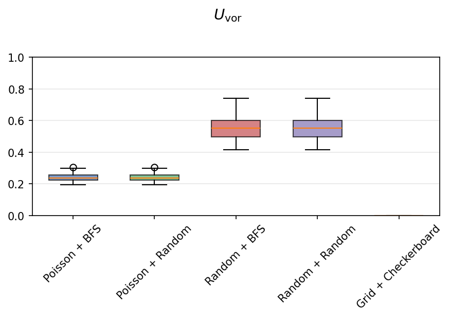
Voronoi Cell Area CV $U_{\mathrm{vor}}$
The coefficient of variation (CV) of Voronoi cell areas measures spatial uniformity of tile placement: $$U_{\mathrm{vor}} = \frac{\sigma_A}{\bar{A}}$$ where $A_i$ is the area of the Voronoi cell for tile $i$, clipped to the region boundary. $U_{\mathrm{vor}} = 0$ for a perfect lattice (all cells identical); $U_{\mathrm{vor}} \approx 0.53$ for a Poisson process (completely random); Poisson-disk sampling yields intermediate values. This is a standard measure in spatial statistics for point pattern analysis (Okabe et al., Spatial Tessellations, 2000). Lower values indicate more uniform tile distribution.
4. Method
With the quality metrics defined above, we now describe the proposed algorithm and the baseline conditions designed to isolate the contribution of each component. The algorithm has two stages — tile placement and angle assignment — and we compare two strategies for each, yielding a 2×2 factorial design.
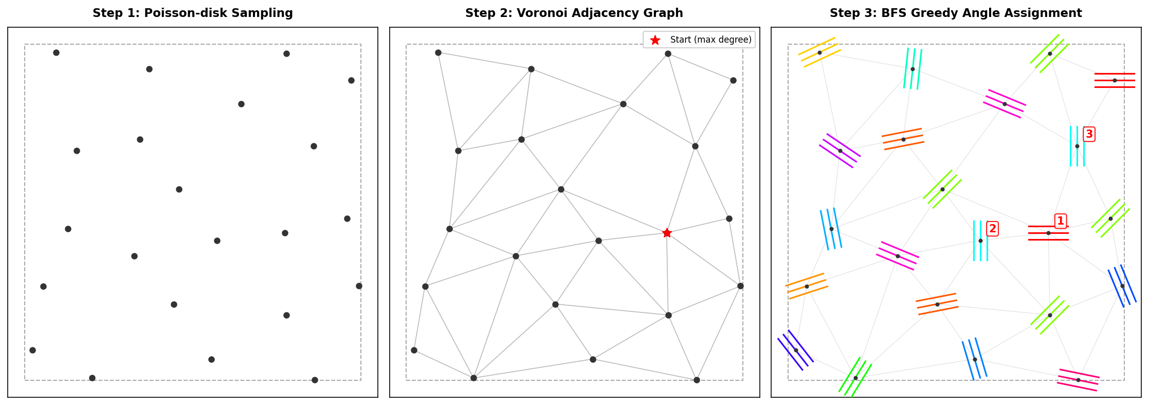
4.1 Algorithm Pipeline Overview
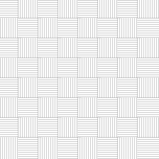
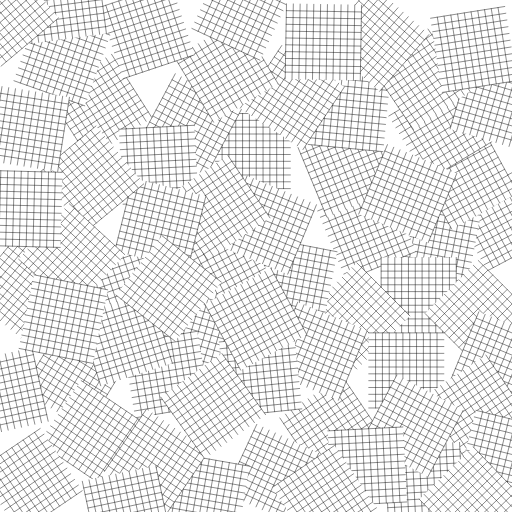
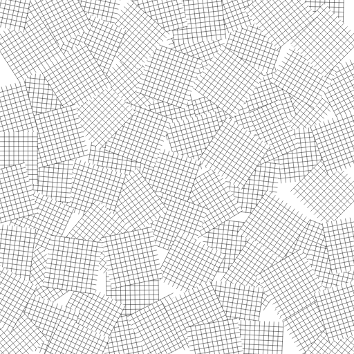
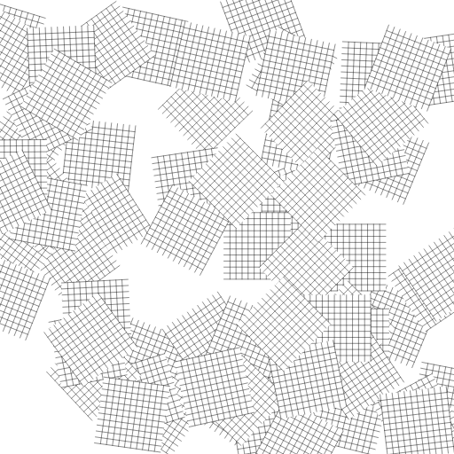
Figure 1 illustrates the three stages of the proposed method: (1) Poisson-disk sampling generates well-spaced tile centres, (2) Delaunay triangulation constructs the Voronoi adjacency graph, and (3) BFS greedy traversal assigns angles that maximise local contrast.
4.2 Tile Placement Strategies
Poisson-disk (Bridson's algorithm): generates well-spaced points with a minimum distance guarantee ($r = \texttt{tileSize}$), producing blue noise spatial distribution. The resulting points serve as tile centres, and a Voronoi adjacency graph is constructed via Delaunay triangulation.
Uniform random: $n$ points drawn from $\mathrm{Uniform}([x_{\min}, x_{\max}] \times [y_{\min}, y_{\max}])$. The count $n$ is matched to the Poisson-disk output for the same seed, ensuring a fair comparison.
4.3 Angle Assignment Strategies
BFS greedy: Starting from the highest-degree node in the adjacency graph, a breadth-first search visits all nodes. For each visited node, 360 candidate angles $\{0, \pi/360, 2\pi/360, \ldots\}$ are evaluated, and the angle maximising $\min_{j \in N_{\mathrm{placed}}} d_{\mathbb{RP}^1}(\theta, \phi_j)$ is selected.
Random: each tile independently receives $\theta \sim \mathrm{Uniform}(0, \pi)$.
4.4 Experimental Conditions (2×2 + Checkerboard)
| BFS Greedy Angles | Random Angles | |
|---|---|---|
| Poisson-disk Placement | poissonBfs (proposed) | poissonRandom |
| Random Placement | randomBfs | randomRandom (baseline) |
In addition to the 2×2 factorial conditions, we include a fifth condition:
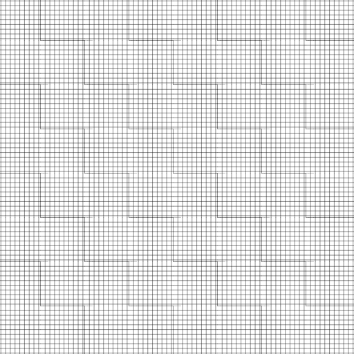
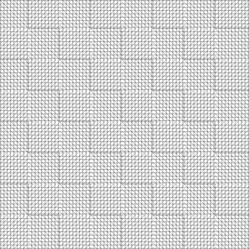
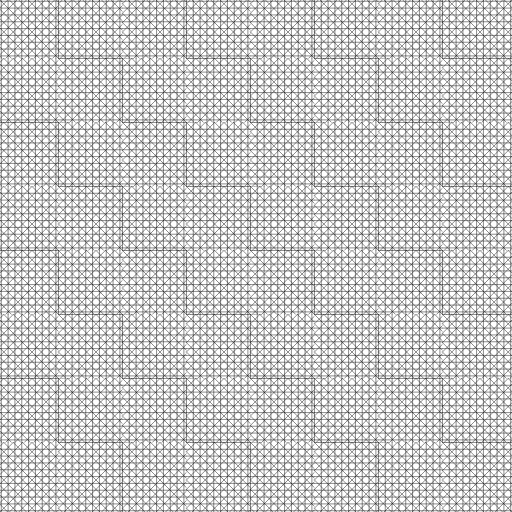
Grid + Checkerboard (gridCheckerboard).
Tiles are placed on an $8 \times 8$ regular square grid (spacing $= 6/8 = 0.75$),
yielding 64 tiles in the $[0, 6]^2$ region —
comparable to the ~69 tiles produced by Poisson-disk sampling.
Angles alternate between 0° and 90° in a checkerboard pattern:
tiles at even $(r + c)$ positions receive 0°, odd positions receive 90°.
This condition is entirely deterministic (identical across all seeds)
and serves as a crystalline order reference:
a periodic pattern that achieves competitive local contrast
and optimal spatial metrics ($C_{\mathrm{cov}} = 1$, $U_{\mathrm{vor}} = 0$),
but exhibits limited angle diversity ($H_{\mathrm{angle}} \approx 0.28$)
and a periodic $R_k$ structure,
producing a visually mechanical, non-natural result.
The $8 \times 8$ grid size was chosen to approximately match the Poisson-disk tile count (~69), enabling fairer comparison of spatial metrics ($C_{\mathrm{cov}}$, $U_{\mathrm{vor}}$).
5. Experimental Setup
To evaluate the five conditions defined in Section 4, we run a controlled experiment with 100 random seeds. All quality metrics are computed at $k = 1$ only, because the metrics ($E_{\mathrm{contrast}}$, $H_{\mathrm{angle}}$, $R_2$, $R_3$) depend solely on the primary angle $\phi_i$ of each tile and are therefore invariant to the kake count $k$. Representative images are rendered at $k = 1, 2, 3, 4$ for the median-$E_{\mathrm{contrast}}$ seed of each condition to illustrate the visual effect of layering.
| Parameter | Value |
|---|---|
| Conditions | 5 (poissonBfs, poissonRandom, randomBfs, randomRandom, gridCheckerboard) |
| $k$ (for metrics) | 1 |
| $k$ (for images) | 1, 2, 3, 4 |
| Seeds | 0–99 (100 seeds) |
| Total runs | $5 \times 100 + 5 \times 3 = 515$ (metrics + extra images) |
| Region | $[0, 0, 6, 6]$ |
| Tile size | 0.6 |
| Pitch | 0.08 |
| Line weight | 0.4 |
| PNG resolution | 512 × 512 |
| Adjacency | Voronoi (Delaunay triangulation of tile centres) |
Rendering uses the same SVG pipeline as the interactive generator, executed in a headless Chromium browser via Playwright for pixel-perfect fidelity. All render noise parameters (angle, spacing, weight) are set to 0 and background hatching is disabled to isolate the effect of placement and angle assignment strategies.
Adjacency consistency. All five conditions use Voronoi adjacency (derived from Delaunay triangulation of tile centres) for both BFS optimisation and metric evaluation. This ensures that the adjacency graph over which the BFS greedy algorithm maximises contrast is identical to the graph used to compute $E_{\mathrm{contrast}}$ and $R_k$.
Software. The generation pipeline is implemented in TypeScript 5.7 with Vite 6.2 as build tool and d3-delaunay 6.0.4 for Voronoi/Delaunay computation. Headless rendering uses Playwright 1.58.2 on Node.js 23.10. Statistical analysis is performed in Python using pandas, NumPy, SciPy, statsmodels, matplotlib, and Jinja2.
6. Results
We present the experimental results using the eight quality metrics defined in Section 3. All metrics are computed at $k = 1$. Section 6.1 shows representative images, Section 6.2 presents box plots and the correlogram, and Section 6.3 provides summary statistics. Full statistical analysis (two-way ANOVA, pairwise effect sizes, and post-hoc tests) is provided in the Appendices.
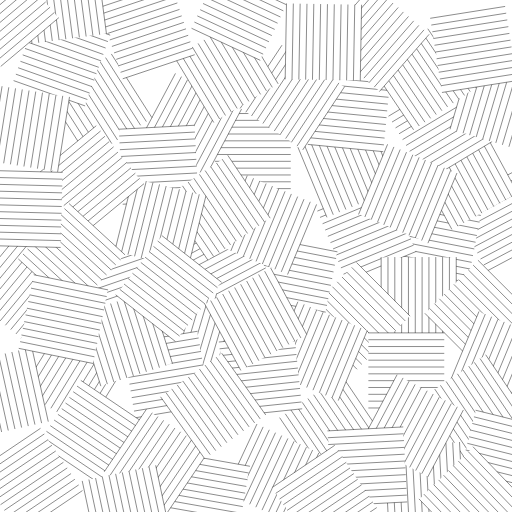
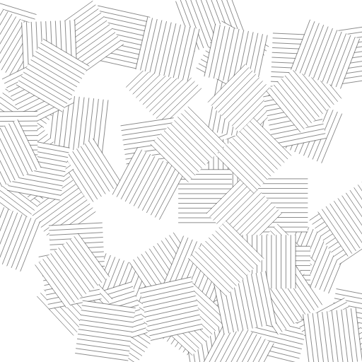
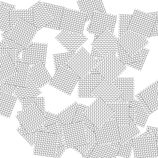
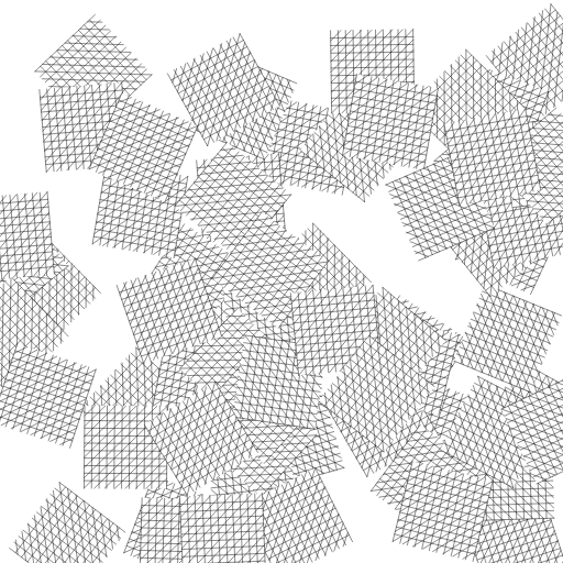
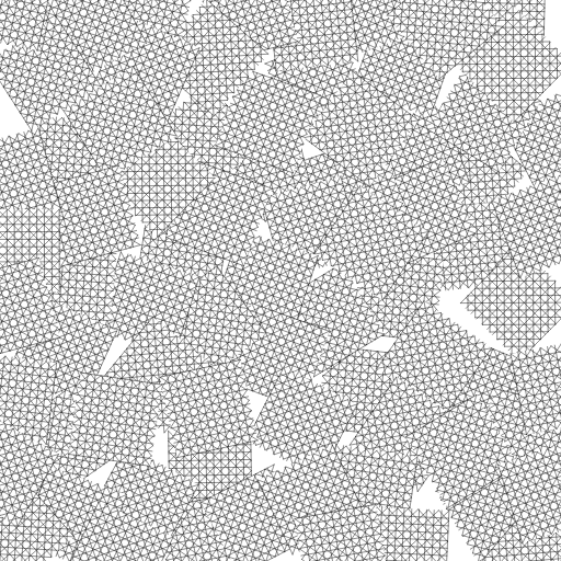
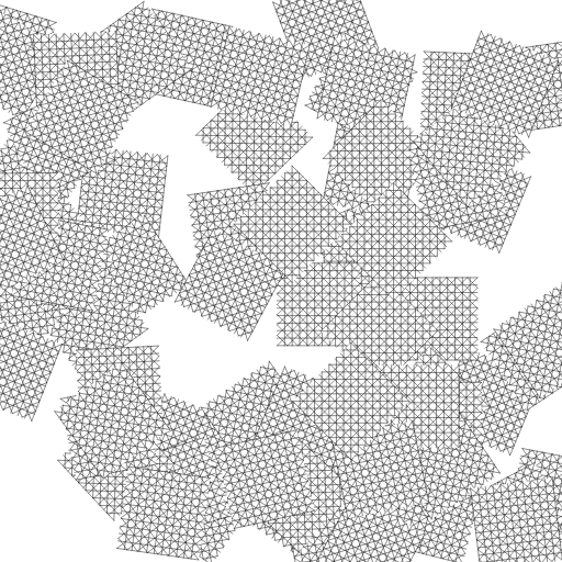
6.1 Representative Images
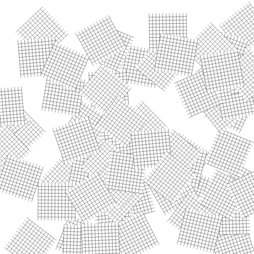
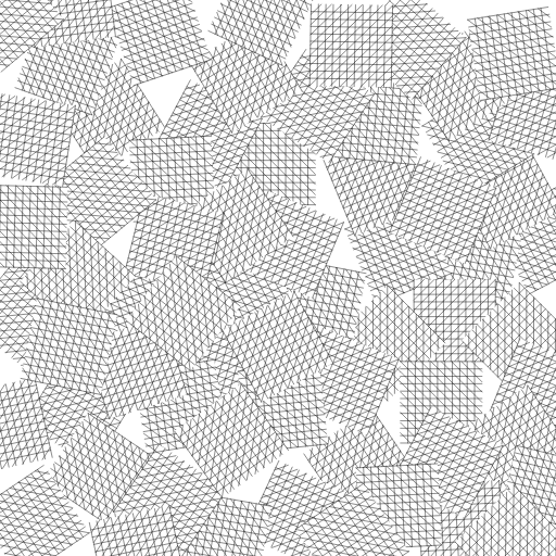
For each condition, the seed whose $E_{\mathrm{contrast}}$ ($k = 1$) is closest to the median is shown. Images are rendered at $k = 1, 2, 3, 4$ to illustrate the visual effect of layering. Note that $k$ does not affect the quality metrics, which depend only on the primary angle $\phi_i$.
$k = 1$
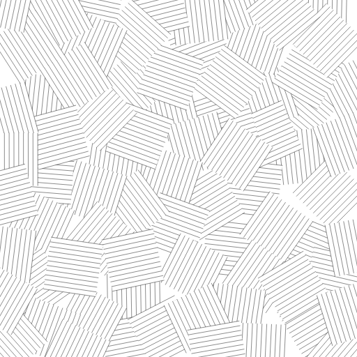

$k = 2$
$k = 3$
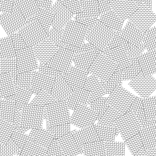
$k = 4$


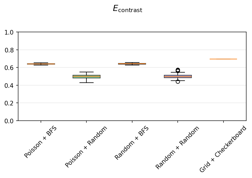
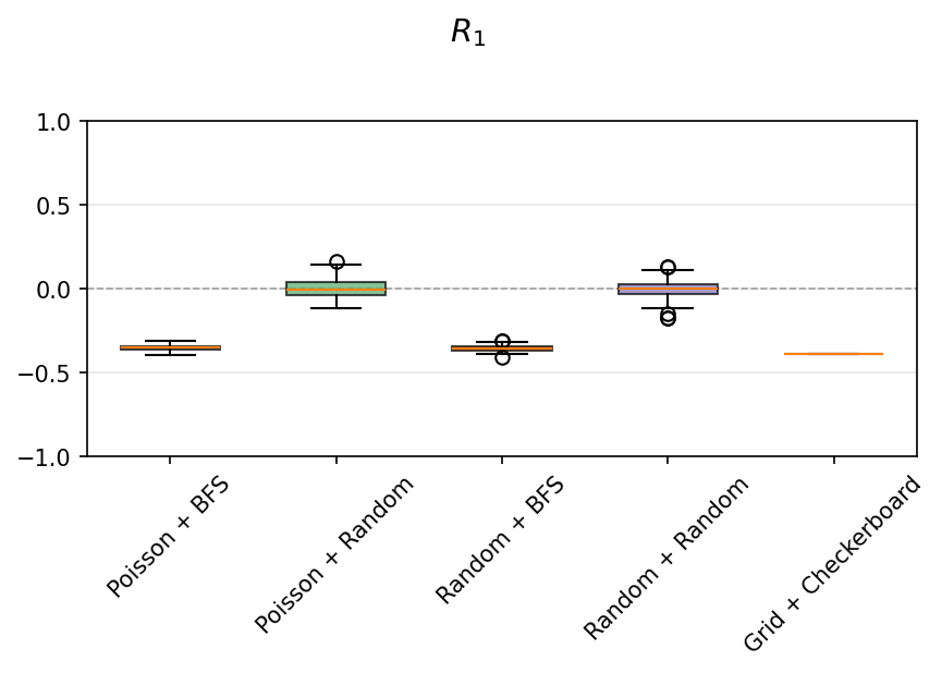
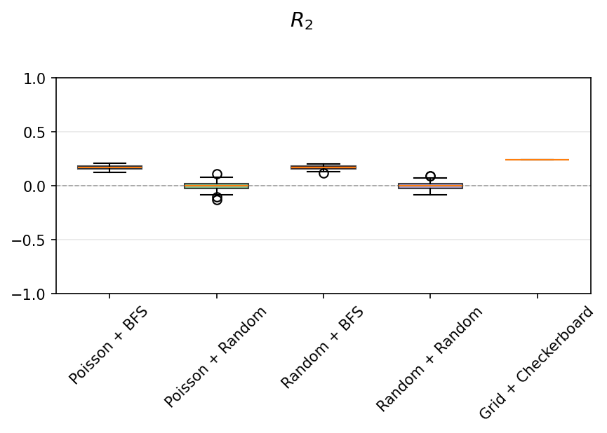
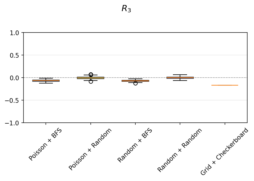
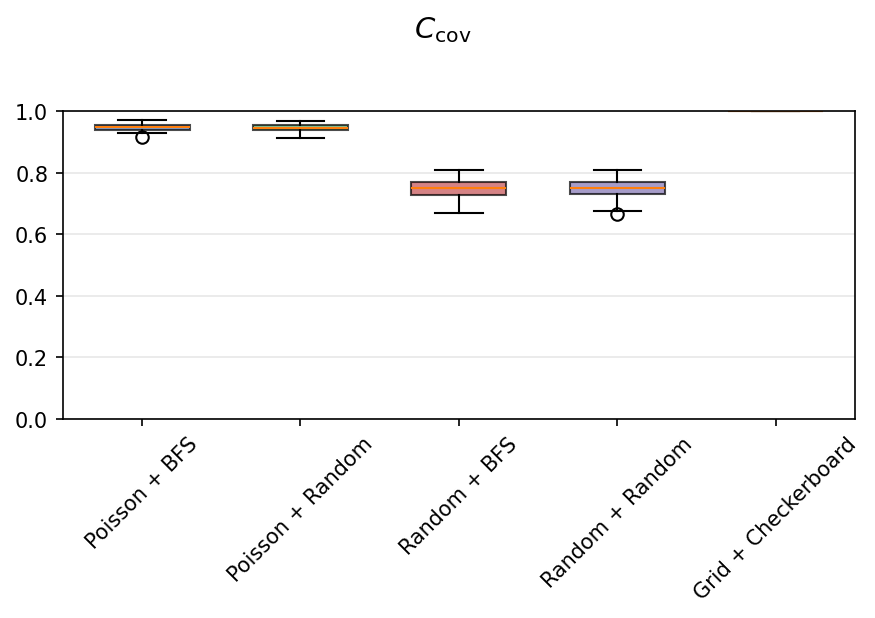
6.2 Quality Metrics
Note: The Grid + Checkerboard condition is a deterministic reference configuration that produces identical results across all seeds (zero variance in the box plots). Its role is discussed in Section 7.4.
6.3 Summary Table
Cells with a dark green background indicate the best-performing condition for that metric; cells with a light green background indicate the second-best condition. Direction: higher is better for $E_{\mathrm{contrast}}$, $H_{\mathrm{angle}}$, and $C_{\mathrm{cov}}$; lower is better for $U_{\mathrm{vor}}$ and $\xi$; $|R_k|$ closest to 0 is best for $R_1$, $R_2$, and $R_3$. All metrics computed at $k = 1$.
| Condition | $E_{\mathrm{contrast}}$ | $H_{\mathrm{angle}}$ | $R_1$ | $R_2$ | $R_3$ | $C_{\mathrm{cov}}$ | $U_{\mathrm{vor}}$ | $\xi$ | Tiles | Edges |
|---|---|---|---|---|---|---|---|---|---|---|
| Poisson + BFS | 0.640 ± 0.005 | 0.960 ± 0.022 | -0.353 ± 0.017 | 0.168 ± 0.017 | -0.067 ± 0.024 | 0.948 ± 0.010 | 0.240 ± 0.021 | 1.305 ± 0.284 | 68.8 | 191.6 |
| Poisson + Random | 0.497 ± 0.026 | 0.968 ± 0.012 | 0.006 ± 0.063 | -0.002 ± 0.040 | -0.004 ± 0.031 | 0.947 ± 0.010 | 0.240 ± 0.021 | 57.439 ± 46.904 | 68.8 | 191.6 |
| Random + BFS | 0.642 ± 0.006 | 0.959 ± 0.023 | -0.358 ± 0.018 | 0.170 ± 0.017 | -0.069 ± 0.020 | 0.749 ± 0.030 | 0.558 ± 0.073 | 1.277 ± 0.206 | 68.8 | 192.1 |
| Random + Random | 0.500 ± 0.023 | 0.967 ± 0.015 | -0.000 ± 0.055 | -0.002 ± 0.037 | -0.002 ± 0.027 | 0.749 ± 0.030 | 0.558 ± 0.073 | 57.682 ± 46.570 | 68.8 | 192.1 |
| Grid + Checkerboard * | 0.696 ± 0.000 | 0.279 ± 0.000 | -0.391 ± 0.000 | 0.241 ± 0.000 | -0.168 ± 0.000 | 1.000 ± 0.000 | 0.000 ± 0.000 | 2.047 ± 0.000 | 64.0 | 161.0 |
* Grid + Checkerboard is a deterministic reference condition outside the 2×2 factorial design. Its role is discussed in Section 7.4.
7. Discussion
The results in Section 6 reveal clear performance differences among the five conditions. Sections 7.1–7.2 analyse the two factors of the 2×2 factorial design, Section 7.3 addresses the central finding — the gap between metric rankings and subjective quality — Section 7.4 discusses the correlation structure revealed by the $R_k$ metrics, Section 7.5 discusses $k$-invariance of the metric framework, and Section 7.6 identifies limitations.
7.1 Effect of Angle Assignment
The two-way ANOVA (Appendix A) confirms that the angle assignment strategy is the dominant factor. For $E_{\mathrm{contrast}}$, the angle factor shows $\eta^2 \approx 0.94$, indicating that BFS greedy assignment accounts for the vast majority of variance in angle contrast. The BFS greedy strategy consistently outperforms random angle assignment on $E_{\mathrm{contrast}}$, confirming that local contrast maximisation via the adjacency graph is the primary driver of angular quality.
7.2 Effect of Tile Placement
While the angular metrics ($E_{\mathrm{contrast}}$, $H_{\mathrm{angle}}$) show little sensitivity to placement strategy, the spatial metrics reveal a stark difference. Poisson-disk placement achieves near-perfect coverage ($C_{\mathrm{cov}} \approx 0.95$) thanks to the 1.4× tile expansion and minimum-distance guarantee, whereas uniform random placement leaves visible gaps ($C_{\mathrm{cov}} \approx 0.75$) due to tile clustering. The Voronoi cell area CV ($U_{\mathrm{vor}}$) confirms this: Poisson-disk conditions show significantly lower CV (more uniform spacing) than random conditions, which approach the theoretical Poisson process value of $\approx 0.53$.
7.3 The Gap Between Metrics and Subjective Quality
A striking result of this experiment is that the proposed Poisson-disk + BFS greedy condition — which produces the most natural-looking kakeami by visual inspection — does not rank first on any of the eight proposed metrics. $E_{\mathrm{contrast}}$ is highest for the checkerboard; $H_{\mathrm{angle}}$ is highest for random-angle conditions; $|R_k|$ closest to zero is achieved by random conditions (which have no angular structure at all); and the spatial metrics ($C_{\mathrm{cov}}$, $U_{\mathrm{vor}}$) are optimal for the deterministic grid.
The subjective quality of Poisson-disk + BFS greedy is characterised by two properties: (1) angular contrast is visible everywhere in the pattern — no local region shows adjacent tiles with similar angles fusing together; and (2) the pattern has a visible grain — the texture looks organic and varied, not mechanical. We term this combination “grain”: the per-tile angular variation is clearly perceptible across the entire field, without any region appearing flat or repetitive.
The proposed metrics fail to capture this property because they are global averages. $E_{\mathrm{contrast}}$ measures the mean pairwise contrast across all edges, but does not penalise a pattern where high average contrast coexists with poor angle diversity (as in the checkerboard, which uses only two angles). $H_{\mathrm{angle}}$ measures angle diversity globally but says nothing about whether diverse angles are arranged to contrast locally (random conditions achieve high $H_{\mathrm{angle}}$ while lacking consistent local contrast). The $R_k$ metrics detect periodicity and long-range correlation, but $R_k \approx 0$ for random conditions simply reflects the absence of any structure, not the presence of well-designed aperiodicity.
No simple weighted combination of the eight metrics resolves this issue: any weighting that favours $E_{\mathrm{contrast}}$ elevates the checkerboard; any weighting that favours $H_{\mathrm{angle}}$ elevates the random conditions. The “grain” quality emerges from the simultaneous achievement of high local contrast, high angle diversity, and spatial regularity — a conjunction that no individual metric or linear combination captures. Developing a metric that aligns with subjective kakeami quality remains an open problem.
7.4 Correlation Structure
The $R_k$ correlogram (Figure 10) reveals three qualitatively distinct regimes. The checkerboard oscillates with period 2 ($R_k \approx (-1)^k$), never decaying — the hallmark of crystalline periodicity. Its low angle diversity ($H_{\mathrm{angle}} \approx 0.28$, using only 2 of 12 angle bins) remains the clearest discriminator of its mechanical character. Random conditions produce a flat correlogram near zero at all distances: no angular structure at any scale. BFS greedy conditions show strong negative $R_1$ decaying rapidly to near-zero by $k = 3$–$4$, with a mild positive $R_2 \approx 0.17$ reflecting the structural side effect of greedy maximisation (tiles at distance 2 share an intermediate neighbour that constrains both their angles).
The correlation length $\xi$ quantifies this decay. BFS conditions achieve small $\xi$ values ($\approx 1$–$2$), indicating angular correlations confined to the immediate neighbourhood. The checkerboard produces $\xi = \infty$ (the exponential decay model fails for oscillatory profiles), and random conditions produce large $\xi$ values ($\approx 57$) because the near-zero $|R_k|$ profile lacks any decay to fit — a model artefact, not evidence of long-range correlation. In both cases, $\xi$ is outside the model’s domain rather than a quantitative measurement (see Section 3.3).
This three-way separation — periodic, frustrated short-range order, and amorphous — is reminiscent of orientational order classifications in condensed matter physics, though the analogy remains informal (see Section 8.5). The BFS conditions occupy the frustrated short-range order region of this space.
7.5 $k$-Invariance of Quality Metrics
All eight metrics depend only on the primary angle $\phi_i$ of each tile and are therefore invariant to the kake count $k$. The secondary strokes added for $k \geq 2$ (at fixed angular offsets of 45°, 90°, etc.) do not influence any of the metrics. This means the metrics cannot distinguish between a $k = 1$ and $k = 4$ configuration that share the same primary angles, even though they look very different visually. We acknowledge this as a gap and propose $k$-aware metrics as future work (Section 8.6).
7.6 Limitations
- Metrics do not capture subjective quality. The proposed condition does not rank first on any metric. The gap between metric rankings and visual quality is the most significant limitation of this work (Section 7.3).
- All evaluation is metric-based. A human perceptual study would strengthen the conclusions.
- The experiment uses a single region size and tile size. Scalability to larger regions has not been tested.
- The 360-candidate grid for BFS is a discretisation; finer grids or continuous optimisation may improve results marginally.
- The quality metrics are $k$-invariant: they capture only primary-angle structure and cannot evaluate the visual contribution of secondary hatch layers (see Section 7.5).
- All conditions use Voronoi adjacency derived from Delaunay triangulation of tile centres. Other adjacency definitions (e.g. $k$-nearest-neighbours or radius-based) remain unexplored.
- The exponential decay model for $\xi$ has not been validated against alternative decay models. $R^2 \approx 0.7$ for BFS conditions indicates acceptable but imperfect fit (see Appendix A).
- ANOVA assumptions (normality, homoscedasticity) are violated for most metrics (Shapiro–Wilk and Levene’s tests significant; see Appendix A). The large sample size ($n = 100$ per condition) provides robustness, but nonparametric alternatives have not been applied.
8. Future Work
The experiment framework and quality metrics established in this report open several directions for future research.
8.1 Perceptually Aligned Quality Metrics
The most pressing open problem identified by this work is the gap between proposed metrics and subjective quality (Section 7.3). The proposed Poisson-disk + BFS greedy condition does not rank first on any of the eight metrics, yet it produces the most natural-looking kakeami by visual inspection. The key unmeasured property is “grain” — the simultaneous achievement of local angular contrast, angle diversity, and spatial regularity that no individual metric or linear combination captures.
Several directions may bridge this gap. A minimum-edge-contrast metric (e.g. the 5th percentile of per-edge $d_{\mathbb{RP}^1}$) would penalise patterns where some adjacent tiles fuse due to similar angles, directly targeting the “no fusion” property. A joint metric that multiplies or thresholds $E_{\mathrm{contrast}}$ and $H_{\mathrm{angle}}$ simultaneously could exclude conditions that score high on one axis but low on the other. Most directly, a human perceptual study — pairwise preference judgements across conditions — would establish ground truth for what “good kakeami” means and enable metric validation or learned composite scores.
8.2 Tonal Gradation via Spatially Varying $k$
In traditional manga practice, artists create smooth tonal gradients by varying the kake count $k$ across a region — transitioning, for example, from 1-kake (lightest) to 4-kake (darkest) to depict the curvature of a face or the fall of shadow. Our current implementation uses a uniform $k$ across all tiles. A natural extension is to accept a scalar field $k(x, y)$ that maps spatial position to kake count, enabling automatic kakeami gradation. The quality metrics defined in Section 3 would need to be extended to handle heterogeneous $k$ values, e.g. by weighting edge contrast contributions by the local $k$.
8.3 Generalisation to Arbitrary Pattern Tiles
A key insight of this work is that the proposed algorithm is pattern-agnostic along two independent axes: the fill content drawn inside each tile, and the tile shape itself. The Poisson-disk placement, Voronoi adjacency construction, and BFS greedy angle assignment operate solely on tile centres and primary angles — neither the rendering primitive nor the tile boundary geometry participates in the optimisation. This opens two complementary directions for generalisation.
8.3.1 Non-Line Fill Patterns in Rectangular Tiles
The rectangular tile shape can be preserved while replacing straight-line hatching with a fundamentally different fill primitive. For example, placing dots along the hatch-line positions at regular intervals produces a stipple pattern whose directional alignment reveals the tile’s primary angle without drawing any continuous line. Other candidates include small crosses, short dashes, concentric arcs, or any oriented motif. Because the fill is independent of the placement framework, the same quality metrics ($E_{\mathrm{contrast}}$, $H_{\mathrm{angle}}$, $R_k$) remain valid: they depend only on the primary angle $\phi_i$ of each tile, not on how that angle is visually manifested inside the tile.

8.3.2 Non-Rectangular Tile Shapes
Independently of the fill content, the tile shape itself can be generalised. Our algorithm already computes a Voronoi partition internally to determine tile adjacency; the Voronoi cells themselves are natural, non-rectangular tile candidates. Each Voronoi cell is an individual kakeami unit: the BFS greedy algorithm assigns an angle to each cell, and the cell polygon is hatched directly — without grouping multiple non-rectangular shapes into a rectangular container. Other tile geometries (regular hexagons, triangles, Penrose rhombi, etc.) are equally viable, as long as an adjacency graph can be constructed.

Together, these two axes of generalisation suggest that the quality metrics and optimisation framework introduced in this work are applicable to a broad class of oriented tile-based texture synthesis problems — any setting where a surface must be covered by directed pattern units with maximal local angular contrast.
8.4 Nawaami (Curved-Line Hatching)
Nawaami (ナワアミ, also called kakenawa カケナワ, literally “rope net”) is a related manga technique that replaces straight hatching lines with curved, sinuous strokes bundled within trapezoidal guide shapes. These curved bundles chain together to form flowing, rope-like textures that convey emotional qualities distinct from standard kakeami — particularly anxiety, unease, and foreboding (Emiya Manga Class). Extending our generation algorithm to nawaami would require replacing the straight-line hatch primitives with parametric curves (e.g. sine-modulated paths or splines) while preserving the tile-based placement and adjacency-optimised angle assignment. The quality metrics could be adapted by defining an analogous RP¹ distance on the tangent direction of curved strokes at tile boundaries.
8.5 Spectral Analysis and Theoretical Bounds
With the correlation length $\xi$ now established as a concrete measure of angular order (Section 7.4), several theoretical directions remain open. The angular power spectrum $\hat{R}(\omega) = \sum_k R_k e^{-i\omega k}$ would provide a frequency-domain characterisation: a flat spectrum for amorphous order, a sharp peak at $\omega = \pi$ for checkerboard periodicity, and a broad low-frequency hump for the frustrated short-range order BFS conditions.
Proving bounds on $R_k$ for BFS greedy on Poisson-Voronoi graphs is a natural next step. The angle assignment problem can be viewed as continuous graph colouring with repulsive constraints, relating it to the circular chromatic number $\chi_c(G)$. For Poisson-Voronoi graphs (expected chromatic number $\approx 4$), tight bounds on $\xi$ as a function of graph topology would formalise the connection between spatial statistics and frustrated short-range order.
8.6 $k$-Aware Quality Metrics
As discussed in Section 7.5, the current metrics are $k$-invariant — they depend only on the primary angle and cannot evaluate the visual contribution of secondary hatch layers. Future work should develop metrics that capture $k$-dependent properties, such as the visual density contrast between adjacent tiles at different $k$ values, the uniformity of angular coverage within each tile, or perceptual texture similarity measures (e.g. SSIM-based comparisons between generated and reference kakeami patterns at each $k$ level).
9. Conclusion
This report presented the first mathematical formulation of kakeami quality and a controlled experiment evaluating tile placement and angle assignment strategies. The proposed Poisson-disk + BFS greedy algorithm produces kakeami that is subjectively the most natural among all tested conditions — achieving angular contrast and visible “grain” throughout the pattern without mechanical repetition.
However, none of the eight proposed quality metrics ranks this condition first. $E_{\mathrm{contrast}}$ favours the checkerboard; $H_{\mathrm{angle}}$ favours random angles; and $R_k \approx 0$ is trivially achieved by random conditions lacking any structure. The metrics are useful for ablation — the 2×2 factorial ANOVA confirms that angle assignment is the dominant factor ($\eta^2 \approx 0.94$) and Poisson-disk placement provides superior spatial uniformity — but they do not capture the holistic quality that makes one kakeami pattern look better than another.
The core open problem is defining a metric for “grain” — the simultaneous achievement of local angular contrast, angle diversity, and spatial regularity that characterises natural-looking kakeami. The $R_k$ correlogram offers a partial path forward, separating conditions into periodic, frustrated short-range order, and amorphous regimes, but it does not directly measure visual quality. Future work includes tonal gradation via spatially varying $k$, generalisation to arbitrary tile shapes and fill patterns, and — most critically — development of a quality metric that agrees with human visual judgement.
10. References
- Praun, E., Hoppe, H., Webb, M., & Finkelstein, A. (2001). Real-Time Hatching. SIGGRAPH 2001.
- Hertzmann, A., & Zorin, D. (2000). Illustrating Smooth Surfaces. SIGGRAPH 2000.
- Xie, H., et al. (2020). ScreenVAE: Automatic Manga Screentone Translation. SIGGRAPH Asia 2020.
- Zhang, L., et al. (2021). Generating Manga from Illustrations. CVPR 2021.
- Conway, J. H., & Radin, C. (1998). Quaquaversal tilings and rotations. Inventiones Mathematicae, 132(1), 179–188.
- Grünbaum, B., & Shephard, G. C. (1987). Tilings and Patterns. W. H. Freeman.
- Secord, A. (2002). Weighted Voronoi Stippling. NPAR 2002, 37–43.
- Okabe, A., Boots, B., Sugihara, K., & Chiu, S. N. (2000). Spatial Tessellations: Concepts and Applications of Voronoi Diagrams (2nd ed.). Wiley.
- Beaufort, P.-A., Lambrechts, J., Henrotte, F., Geuzaine, C., & Remacle, J.-F. (2017). Computing cross fields — A PDE approach based on the Ginzburg-Landau theory. arXiv:1706.01344.
- Viertel, R., & Osting, B. (2019). An Approach to Quad Meshing Based on Harmonic Cross-Valued Maps and the Ginzburg-Landau Theory. SIAM J. Sci. Comput., 41(1).
- Vaxman, A., et al. (2016). Directional Field Synthesis, Design, and Processing. Computer Graphics Forum, 35(2), 545–572.
- カケアミ. Pixiv Encyclopedia. https://dic.pixiv.net/a/カケアミ.
- Toudo, R. (2003). マンガの基礎デッサン [Manga Basic Drawing]. Hobby Japan.
- Japanese with Anime. (2020). Kakeami. www.japanesewithanime.com/2020/03/kakeami.html.
- Emiya Manga Class. (2018). カケアミの描き方. lanmy.net/2018/05/manga-kakeami/.
- Shechtman, D., Blech, I., Gratias, D., & Cahn, J. W. (1984). Metallic phase with long-range orientational order and no translational symmetry. Physical Review Letters, 53(20), 1951–1953.
- de Gennes, P.-G., & Prost, J. (1993). The Physics of Liquid Crystals (2nd ed.). Oxford University Press.
- Cressie, N. (1993). Statistics for Spatial Data (Revised ed.). Wiley.
- Cliff, A. D., & Ord, J. K. (1981). Spatial Processes: Models & Applications. Pion.
- Toulouse, G. (1977). Theory of the frustration effect in spin glasses. Communications on Physics, 2, 115–119.
Appendix A. Two-Way ANOVA Tables
Two-way ANOVA (Type II) with placement and angle as fixed factors. Only the four 2×2 factorial conditions are included (gridCheckerboard is excluded). $\eta^2$ and bias-corrected $\omega^2$ are reported as effect size measures. Assumption tests (Shapiro–Wilk for normality of residuals, Levene’s test for homoscedasticity) are reported below each table. No correction for multiple testing across metrics is applied.
ANOVA: $E_{\mathrm{contrast}}$
| Source | SS | df | $F$ | $p$ | $\eta^2$ | $\omega^2$ |
|---|---|---|---|---|---|---|
| Placement | 0.000455 | 1 | 1.47 | 0.2261 | 0.0002 | 0.0001 |
| Angle | 2.014764 | 1 | 6512.32 | 0.0000 | 0.9425 | 0.9422 |
| Placement × Angle | 0.000023 | 1 | 0.07 | 0.7872 | 0.0000 | 0.0000 |
| Residual | 0.122513 | 396 | — | — | 0.0573 | — |
Assumption tests — Shapiro–Wilk: $W = 0.9255$, $p = 0.0000$; Levene: $F = 55.9992$, $p = 0.0000$.
ANOVA: $H_{\mathrm{angle}}$
| Source | SS | df | $F$ | $p$ | $\eta^2$ | $\omega^2$ |
|---|---|---|---|---|---|---|
| Placement | 0.000115 | 1 | 0.34 | 0.5609 | 0.0008 | 0.0000 |
| Angle | 0.006915 | 1 | 20.29 | 0.0000 | 0.0487 | 0.0462 |
| Placement × Angle | 0.000002 | 1 | 0.01 | 0.9331 | 0.0000 | 0.0000 |
| Residual | 0.134947 | 396 | — | — | 0.9505 | — |
Assumption tests — Shapiro–Wilk: $W = 0.9308$, $p = 0.0000$; Levene: $F = 8.7589$, $p = 0.0000$.
ANOVA: $R_1$
| Source | SS | df | $F$ | $p$ | $\eta^2$ | $\omega^2$ |
|---|---|---|---|---|---|---|
| Placement | 0.002996 | 1 | 1.57 | 0.2111 | 0.0002 | 0.0001 |
| Angle | 12.813288 | 1 | 6710.04 | 0.0000 | 0.9441 | 0.9438 |
| Placement × Angle | 0.000040 | 1 | 0.02 | 0.8849 | 0.0000 | 0.0000 |
| Residual | 0.756189 | 396 | — | — | 0.0557 | — |
Assumption tests — Shapiro–Wilk: $W = 0.9433$, $p = 0.0000$; Levene: $F = 44.2606$, $p = 0.0000$.
ANOVA: $C_{\mathrm{cov}}$
| Source | SS | df | $F$ | $p$ | $\eta^2$ | $\omega^2$ |
|---|---|---|---|---|---|---|
| Placement | 3.942295 | 1 | 7823.87 | 0.0000 | 0.9518 | 0.9516 |
| Angle | 0.000008 | 1 | 0.02 | 0.9001 | 0.0000 | 0.0000 |
| Placement × Angle | 0.000017 | 1 | 0.03 | 0.8543 | 0.0000 | 0.0000 |
| Residual | 0.199537 | 396 | — | — | 0.0482 | — |
Assumption tests — Shapiro–Wilk: $W = 0.9667$, $p = 0.0000$; Levene: $F = 47.7260$, $p = 0.0000$.
ANOVA: $U_{\mathrm{vor}}$
| Source | SS | df | $F$ | $p$ | $\eta^2$ | $\omega^2$ |
|---|---|---|---|---|---|---|
| Placement | 10.119846 | 1 | 3465.56 | 0.0000 | 0.8975 | 0.8970 |
| Angle | 0.000000 | 1 | 0.00 | 1.0000 | 0.0000 | 0.0000 |
| Placement × Angle | 0.000000 | 1 | 0.00 | 1.0000 | 0.0000 | 0.0000 |
| Residual | 1.156367 | 396 | — | — | 0.1025 | — |
Assumption tests — Shapiro–Wilk: $W = 0.9529$, $p = 0.0000$; Levene: $F = 54.8041$, $p = 0.0000$.
ANOVA: $R_2$
| Source | SS | df | $F$ | $p$ | $\eta^2$ | $\omega^2$ |
|---|---|---|---|---|---|---|
| Placement | 0.000135 | 1 | 0.15 | 0.6972 | 0.0000 | 0.0000 |
| Angle | 2.920270 | 1 | 3268.69 | 0.0000 | 0.8918 | 0.8913 |
| Placement × Angle | 0.000244 | 1 | 0.27 | 0.6013 | 0.0001 | 0.0000 |
| Residual | 0.353789 | 396 | — | — | 0.1080 | — |
Assumption tests — Shapiro–Wilk: $W = 0.9741$, $p = 0.0000$; Levene: $F = 25.1803$, $p = 0.0000$.
ANOVA: $R_3$
| Source | SS | df | $F$ | $p$ | $\eta^2$ | $\omega^2$ |
|---|---|---|---|---|---|---|
| Placement | 0.000000 | 1 | 0.00 | 0.9844 | 0.0000 | 0.0000 |
| Angle | 0.426088 | 1 | 647.16 | 0.0000 | 0.6200 | 0.6185 |
| Placement × Angle | 0.000398 | 1 | 0.60 | 0.4372 | 0.0006 | 0.0000 |
| Residual | 0.260723 | 396 | — | — | 0.3794 | — |
Assumption tests — Shapiro–Wilk: $W = 0.9953$, $p = 0.2674$; Levene: $F = 4.0526$, $p = 0.0074$.
ANOVA: $\xi$
| Source | SS | df | $F$ | $p$ | $\eta^2$ | $\omega^2$ |
|---|---|---|---|---|---|---|
| Placement | 1.141877 | 1 | 0.00 | 0.9742 | 0.0000 | 0.0000 |
| Angle | 316624.747489 | 1 | 289.89 | 0.0000 | 0.4226 | 0.4206 |
| Placement × Angle | 1.837482 | 1 | 0.00 | 0.9673 | 0.0000 | 0.0000 |
| Residual | 432518.103745 | 396 | — | — | 0.5773 | — |
Assumption tests — Shapiro–Wilk: $W = 0.8264$, $p = 0.0000$; Levene: $F = 54.5177$, $p = 0.0000$.
Goodness of Fit for $\xi$ (Exponential Decay Model)
Mean $R^2$ values for the per-seed exponential decay fit $|R_k| \approx A \exp(-k/\xi)$:
| Condition | Mean $R^2$ |
|---|---|
| Poisson + BFS | 0.730 |
| Poisson + Random | -0.124 |
| Random + BFS | 0.691 |
| Random + Random | -0.149 |
| Grid + Checkerboard | -0.384 |
$R^2 \approx 0.7$ for BFS conditions indicates acceptable but imperfect fit. Negative $R^2$ for random and checkerboard conditions indicates model inapplicability (see Section 3.3 caveats). Alternative decay models (e.g. power-law $|R_k| \sim k^{-\alpha}$) have not been compared.
Appendix B. Pairwise Effect Sizes (Cohen’s $d$)
Cohen’s $d$ (pooled SD) for the four factorial conditions (6 pairs); the deterministic gridCheckerboard condition is excluded. Positive $d$ indicates the first condition scores higher than the second. By convention: $|d| < 0.2$ negligible, $0.2$–$0.5$ small, $0.5$–$0.8$ medium, $> 0.8$ large.
$E_{\mathrm{contrast}}$
| Pair | Cohen's $d$ |
|---|---|
| Poisson + BFS vs Poisson + Random | 7.654 |
| Poisson + BFS vs Random + BFS | -0.305 |
| Poisson + BFS vs Random + Random | 8.509 |
| Poisson + Random vs Random + BFS | -7.714 |
| Poisson + Random vs Random + Random | -0.107 |
| Random + BFS vs Random + Random | 8.570 |
$H_{\mathrm{angle}}$
| Pair | Cohen's $d$ |
|---|---|
| Poisson + BFS vs Poisson + Random | -0.480 |
| Poisson + BFS vs Random + BFS | 0.042 |
| Poisson + BFS vs Random + Random | -0.387 |
| Poisson + Random vs Random + BFS | 0.516 |
| Poisson + Random vs Random + Random | 0.089 |
| Random + BFS vs Random + Random | -0.424 |
$R_1$
| Pair | Cohen's $d$ |
|---|---|
| Poisson + BFS vs Poisson + Random | -7.746 |
| Poisson + BFS vs Random + BFS | 0.276 |
| Poisson + BFS vs Random + Random | -8.684 |
| Poisson + Random vs Random + BFS | 7.799 |
| Poisson + Random vs Random + Random | 0.103 |
| Random + BFS vs Random + Random | -8.729 |
$C_{\mathrm{cov}}$
| Pair | Cohen's $d$ |
|---|---|
| Poisson + BFS vs Poisson + Random | 0.069 |
| Poisson + BFS vs Random + BFS | 8.987 |
| Poisson + BFS vs Random + Random | 8.780 |
| Poisson + Random vs Random + BFS | 8.912 |
| Poisson + Random vs Random + Random | 8.709 |
| Random + BFS vs Random + Random | -0.004 |
$U_{\mathrm{vor}}$
| Pair | Cohen's $d$ |
|---|---|
| Poisson + BFS vs Poisson + Random | 0.000 |
| Poisson + BFS vs Random + BFS | -5.887 |
| Poisson + BFS vs Random + Random | -5.887 |
| Poisson + Random vs Random + BFS | -5.887 |
| Poisson + Random vs Random + Random | -5.887 |
| Random + BFS vs Random + Random | 0.000 |
$R_2$
| Pair | Cohen's $d$ |
|---|---|
| Poisson + BFS vs Poisson + Random | 5.504 |
| Poisson + BFS vs Random + BFS | -0.157 |
| Poisson + BFS vs Random + Random | 5.844 |
| Poisson + Random vs Random + BFS | -5.602 |
| Poisson + Random vs Random + Random | 0.010 |
| Random + BFS vs Random + Random | 5.949 |
$R_3$
| Pair | Cohen's $d$ |
|---|---|
| Poisson + BFS vs Poisson + Random | -2.296 |
| Poisson + BFS vs Random + BFS | 0.089 |
| Poisson + BFS vs Random + Random | -2.584 |
| Poisson + Random vs Random + BFS | 2.505 |
| Poisson + Random vs Random + Random | -0.071 |
| Random + BFS vs Random + Random | -2.849 |
$xi$
| Pair | Cohen's $d$ |
|---|---|
| Poisson + BFS vs Poisson + Random | -1.692 |
| Poisson + BFS vs Random + BFS | 0.116 |
| Poisson + BFS vs Random + Random | -1.712 |
| Poisson + Random vs Random + BFS | 1.693 |
| Poisson + Random vs Random + Random | -0.005 |
| Random + BFS vs Random + Random | -1.713 |
Appendix C. Tukey HSD Post-Hoc Comparisons
Tukey’s Honestly Significant Difference test ($\alpha = 0.05$) for the four factorial conditions (6 pairwise comparisons per metric). “Reject” indicates that the mean difference is statistically significant after correction for multiple comparisons within each metric.
$E_{\mathrm{contrast}}$
| Group 1 | Group 2 | Mean Diff | $p$-adj | Lower | Upper | Reject |
|---|---|---|---|---|---|---|
| Poisson + BFS | Poisson + Random | -0.1424 | 0.0000 | -0.1488 | -0.1360 | Yes |
| Poisson + BFS | Random + BFS | 0.0017 | 0.9098 | -0.0048 | 0.0081 | No |
| Poisson + BFS | Random + Random | -0.1398 | 0.0000 | -0.1462 | -0.1334 | Yes |
| Poisson + Random | Random + BFS | 0.1441 | 0.0000 | 0.1377 | 0.1505 | Yes |
| Poisson + Random | Random + Random | 0.0026 | 0.7211 | -0.0038 | 0.0090 | No |
| Random + BFS | Random + Random | -0.1415 | 0.0000 | -0.1479 | -0.1350 | Yes |
$H_{\mathrm{angle}}$
| Group 1 | Group 2 | Mean Diff | $p$-adj | Lower | Upper | Reject |
|---|---|---|---|---|---|---|
| Poisson + BFS | Poisson + Random | 0.0085 | 0.0070 | 0.0017 | 0.0152 | Yes |
| Poisson + BFS | Random + BFS | -0.0009 | 0.9850 | -0.0077 | 0.0058 | No |
| Poisson + BFS | Random + Random | 0.0072 | 0.0295 | 0.0005 | 0.0140 | Yes |
| Poisson + Random | Random + BFS | -0.0094 | 0.0020 | -0.0161 | -0.0027 | Yes |
| Poisson + Random | Random + Random | -0.0012 | 0.9654 | -0.0080 | 0.0055 | No |
| Random + BFS | Random + Random | 0.0082 | 0.0102 | 0.0014 | 0.0149 | Yes |
$R_1$
| Group 1 | Group 2 | Mean Diff | $p$-adj | Lower | Upper | Reject |
|---|---|---|---|---|---|---|
| Poisson + BFS | Poisson + Random | 0.3586 | 0.0000 | 0.3426 | 0.3745 | Yes |
| Poisson + BFS | Random + BFS | -0.0048 | 0.8620 | -0.0208 | 0.0111 | No |
| Poisson + BFS | Random + Random | 0.3525 | 0.0000 | 0.3365 | 0.3684 | Yes |
| Poisson + Random | Random + BFS | -0.3634 | 0.0000 | -0.3794 | -0.3475 | Yes |
| Poisson + Random | Random + Random | -0.0061 | 0.7563 | -0.0221 | 0.0098 | No |
| Random + BFS | Random + Random | 0.3573 | 0.0000 | 0.3414 | 0.3733 | Yes |
$C_{\mathrm{cov}}$
| Group 1 | Group 2 | Mean Diff | $p$-adj | Lower | Upper | Reject |
|---|---|---|---|---|---|---|
| Poisson + BFS | Poisson + Random | -0.0007 | 0.9963 | -0.0089 | 0.0075 | No |
| Poisson + BFS | Random + BFS | -0.1990 | 0.0000 | -0.2072 | -0.1908 | Yes |
| Poisson + BFS | Random + Random | -0.1988 | 0.0000 | -0.2070 | -0.1906 | Yes |
| Poisson + Random | Random + BFS | -0.1983 | 0.0000 | -0.2065 | -0.1901 | Yes |
| Poisson + Random | Random + Random | -0.1981 | 0.0000 | -0.2063 | -0.1899 | Yes |
| Random + BFS | Random + Random | 0.0001 | 1.0000 | -0.0081 | 0.0083 | No |
$U_{\mathrm{vor}}$
| Group 1 | Group 2 | Mean Diff | $p$-adj | Lower | Upper | Reject |
|---|---|---|---|---|---|---|
| Poisson + BFS | Poisson + Random | 0.0000 | 1.0000 | -0.0197 | 0.0197 | No |
| Poisson + BFS | Random + BFS | 0.3181 | 0.0000 | 0.2984 | 0.3378 | Yes |
| Poisson + BFS | Random + Random | 0.3181 | 0.0000 | 0.2984 | 0.3378 | Yes |
| Poisson + Random | Random + BFS | 0.3181 | 0.0000 | 0.2984 | 0.3378 | Yes |
| Poisson + Random | Random + Random | 0.3181 | 0.0000 | 0.2984 | 0.3378 | Yes |
| Random + BFS | Random + Random | 0.0000 | 1.0000 | -0.0197 | 0.0197 | No |
$R_2$
| Group 1 | Group 2 | Mean Diff | $p$-adj | Lower | Upper | Reject |
|---|---|---|---|---|---|---|
| Poisson + BFS | Poisson + Random | -0.1693 | 0.0000 | -0.1802 | -0.1584 | Yes |
| Poisson + BFS | Random + BFS | 0.0027 | 0.9172 | -0.0082 | 0.0136 | No |
| Poisson + BFS | Random + Random | -0.1697 | 0.0000 | -0.1806 | -0.1588 | Yes |
| Poisson + Random | Random + BFS | 0.1721 | 0.0000 | 0.1611 | 0.1830 | Yes |
| Poisson + Random | Random + Random | -0.0004 | 0.9997 | -0.0113 | 0.0105 | No |
| Random + BFS | Random + Random | -0.1725 | 0.0000 | -0.1834 | -0.1615 | Yes |
$R_3$
| Group 1 | Group 2 | Mean Diff | $p$-adj | Lower | Upper | Reject |
|---|---|---|---|---|---|---|
| Poisson + BFS | Poisson + Random | 0.0633 | 0.0000 | 0.0539 | 0.0726 | Yes |
| Poisson + BFS | Random + BFS | -0.0019 | 0.9502 | -0.0113 | 0.0074 | No |
| Poisson + BFS | Random + Random | 0.0653 | 0.0000 | 0.0560 | 0.0747 | Yes |
| Poisson + Random | Random + BFS | -0.0652 | 0.0000 | -0.0746 | -0.0559 | Yes |
| Poisson + Random | Random + Random | 0.0020 | 0.9427 | -0.0073 | 0.0114 | No |
| Random + BFS | Random + Random | 0.0673 | 0.0000 | 0.0579 | 0.0766 | Yes |
$\xi$
| Group 1 | Group 2 | Mean Diff | $p$-adj | Lower | Upper | Reject |
|---|---|---|---|---|---|---|
| Poisson + BFS | Poisson + Random | 56.1339 | 0.0000 | 44.0756 | 68.1921 | Yes |
| Poisson + BFS | Random + BFS | -0.0287 | 1.0000 | -12.0870 | 12.0296 | No |
| Poisson + BFS | Random + Random | 56.3763 | 0.0000 | 44.3180 | 68.4345 | Yes |
| Poisson + Random | Random + BFS | -56.1626 | 0.0000 | -68.2208 | -44.1043 | Yes |
| Poisson + Random | Random + Random | 0.2424 | 0.9999 | -11.8158 | 12.3007 | No |
| Random + BFS | Random + Random | 56.4050 | 0.0000 | 44.3467 | 68.4632 | Yes |